DATA ANALYSIS
After the cleaning of the file, the data file will be stored in the R directory. The first step in the R is to look after the working directory. The “getwd” function will be used for the aspect. After getting the working directory, it is necessary to upload the file in the particular directory and source the data in the R programming.
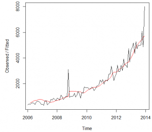
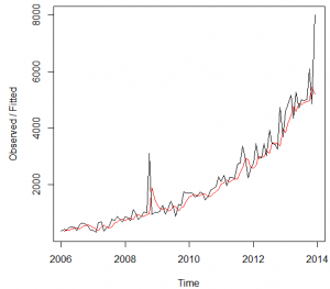
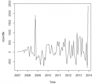
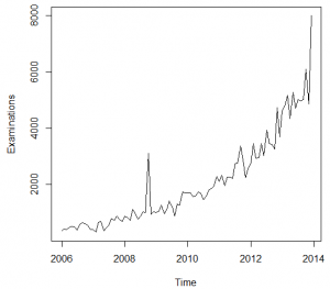
The time series is made accordingly to the data, form the January 2006 to the December 2013 in order to match the given data. The figure 1 below shows the presentation of the data.
Figure 1
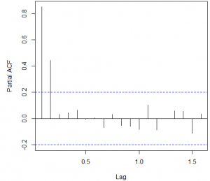
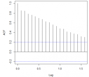
The ultimate boom in the examinations has been observed in the October 2008 that was due to the hurricane in the New Orleans. Before the application of the ARIMA models, it is necessary to analyze the auto regression and moving average with the help of the ACF and PACF graph and integration with the differentiation function. The Figure 2 and 3 below shows the ACF and PACF plots of the time series data.
Figure 2
The ACF function shows the short term relationship between the observations that declares a smooth declining relation has been observed from the data set. The ACF suggests the auto regression (value of p) should be 1 or 2.
Figure 3
The Partial ACF graph is used to analyze the Moving averages used in the data. The PACF graph suggest that the value of q should be 1 or 2 as the PACF shows the long term relationship between the observations. The ADF and Box test were also conducted in order to analyze the data series.
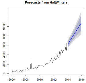
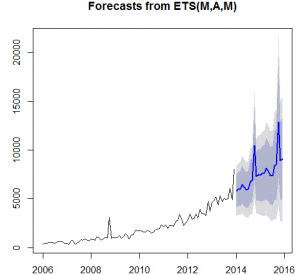
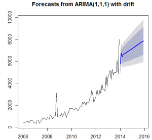
The results from the Box –LJung test shows the significance of the data as the p-value is less than 0.05. However, the Augmented Dickey-Fuller test accepts the alternative hypothesis of the data is stationary. The ARIMA models and Exponential models has been applied on the data set in order to forecast the examinations for the next two years. The three techniques of the ARIMA was used and four techniques of Exponential Smoothing were used.
ARIMA MODEL
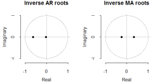
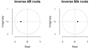
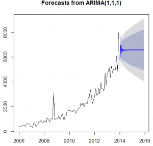
The ARIMA model is used to forecast the future expected values by considering three basic factors of auto correlation, integration and moving averages. The ARIMA model has been applied three times on the data set. The results from the ARIMA models are as follows:
Arima(x = tsdata, order = c (1, 1, 1))
Coefficients:
ar1 ma1
-0.5243 -0.2187
s.e. 0.1708 0.1861
Sigma^2 estimated as 236496: log likelihood = -722.84, aic = 1451.69
Arima(x = tsdata, order = c (2, 1, 2))
Coefficients:
ar1 ar2 ma1 ma2
-0.650 -0.0165 -0.0920 -0.0805
s.e. 1.076 0.6004 1.0712 0.2612
Sigma^2 estimated as 236087: log likelihood = -722.77, aic = 1455.54
Arima (1, 1, 1) with drift
Coefficients:
ar1 ma1 drift
-0.8546 -0.6096 50.5962
s.e. 0.1289 0.1021 14.2494
Sigma^2 estimated as 426397: log likelihood=-750.33
AIC=1508.66 AICc=1509.11 BIC=1518.88
EXPONENTIAL MODEL
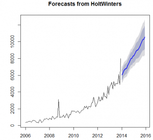
The Exponential model is also a well-known model used in order to forecast future values by considering the growth function at different levels. The auto exponential smoothing, single exponential model, double exponential model and triple exponential model were used in order to forecast the future outcomes. Below are the results of the four exponential models used in the time series data set.
Auto Exponential Model
Ets(y = ts data)
Smoothing parameters:
Alpha = 0.1566 Beta = 0.0135 Gamma = 2e-04
Initial states: l = 390.3993 b = 17.732
s=0.9927 0.9894 1.4527 0.9719 0.9753 0.8724
0.8825 0.9472 1.0083 0.9641 0.9739 0.9697
Sigma: 0.2235
AIC AICc BIC
1584.553 1591.439 1625.582
Single Exponential Model
Length Class Mode
Fitted 190 mts numeric
X 96 ts numeric
Alpha 1 -none- numeric
Beta 1 -none- logical
Gamma 1 -none- logical
Coefficients 1 -none- numeric
Seasonal 1 -none- character
SSE 1 -none- numeric
Call 4 -none- call
Double Exponential Model
Length Class Mode
Fitted 282 mts numeric
X 96 ts numeric
Alpha 1 -none- numeric
Beta 1 -none- numeric
Gamma 1 -none- logical
Coefficients 2 -none- numeric
Seasonal 1 -none- character
SSE 1 -none- numeric
Call 3 -none- call
Triple Exponential Model
Length Class Mode
Fitted 336 mts numeric
X 96 ts numeric
Alpha 1 -none- numeric
Beta 1 -none- numeric
Gamma 1 -none- numeric
Coefficients 14 -none- numeric
Seasonal 1 -none- character
SSE 1 -none- numeric
Call 2 -none- call
Accuracy Comparison and Recommendation
The recommendation is completely based on the efficiency of the model. The Accuracy of the model plays important role when it comes to forecasting. The Accuracy of the model is analyzed by several terms such as Mean Error, Root Mean Square Error, Mean Absolute Error, Mean Percentage Error, Mean Absolute Percentage Error and Mean Absolute Scale Error. Below is the table 1 shows the comparison of three ARIMA models and Auto Exponential Smoothing model.
Table 1
| ARIMA(1,1,1) | ARIMA(2,1,2) | A to Arima | Auto Exponential | |
| ME | -1.87 | 129.14 | -1.87 | 65.44 |
| RMSE | 639.24 | 483.35 | 639.24 | 573.08 |
| MAE | 384.73 | 287.29 | 384.73 | 341.48 |
| MPE | -19.80% | 10.64% | -19.80% | -1.03% |
| MAPE | 33.11% | 23.76% | 33.11% | 17.14% |
| MASE | 0.49 | 0.69 | 0.49 | 0.46 |
It is observed from the above table that the exponential model is assumed as the most effective model as the mean percentage of error in the model is just 1.03 percent as compare to relatively high mean error percentages of 19.8, 10.64 by other models. It is recommended to the Fargo Health to adapt the auto exponential smoothing model in order to forecast the future number of examinations.
Appendix
Examinations
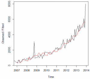
Holt-Winters Filtering